Research note

A Field, Not a Neural Net

The environment error field as a measured physical correction layer for universal machine-learning interatomic potentials.

• July 9, 2026
• ·
• Draft

The dominant narrative in computational materials science is that bigger models trained on more data will close the gap between prediction and synthesis. The evidence points elsewhere. Google DeepMind’s GNoME predicted 2.2 million crystals; only 736 had been independently synthesized by late 2023, a 0.2% validation rate^[1]. The A-Lab Author Correction (Nature 650:E1, 2026) records 36 confirmed of 57 eligible targets, with 4 inconclusive and one compound removed for training-data leakage; a separate critique disputed the novelty classification of many targets^[2]. The problem is not that the models are too small. It is that their errors have a shape — a systematic, low-dimensional geometry in the space of local atomic environments — and the field has been treating that shape as noise.

The present approach starts from the opposite premise. The wrongness of universal machine-learning interatomic potentials (uMLIPs) is not random. It is a smooth function of coordination number, measurable from a handful of anchor observables, and correctable at runtime with analytic forces. The environment error field is the focus: what it is, how it is measured rather than learned, and why the distinction matters for climate-critical materials discovery.

The Field Hypothesis

A uMLIP such as CHGNet, MACE-MP-0, or M3GNet evaluates atomic energies in milliseconds, enabling screening campaigns that would be economically impossible with density functional theory (DFT). On bulk formation energies the best models reach mean absolute errors of 29–81 meV/atom, close to the intrinsic accuracy of the DFT functionals on which they were trained^[3]. But functional materials do not operate as bulk crystals. Ion conduction, catalytic turnover, and hydrolytic stability all depend on under-coordinated environments — vacancies, surfaces, and transition states — where uMLIPs fail most severely: defect formation energies carry large percentage errors, and ion migration barriers are underestimated by more than 60%^[4].

The error is not an inescapable property of machine learning. It is a predictable consequence of training data. Databases such as the Materials Project trajectories, OMat24, and Alexandria are dominated by near-equilibrium, closed-shell bulk structures in which every atom sits close to its high-symmetry coordination. A smooth regressor trained on that distribution interpolates accurately at the bulk coordination but extrapolates with correlated bias into under-coordinated regimes: surfaces, vacancies, transition states, and grain boundaries^[5].

This observation is formalized as the environment error field. For a given configuration, the total systematic energy error of a uMLIP is approximated by a sum over atoms of a per-atom error that depends only on the atom’s local coordination number $c$:

$$E^{\text{model}} - E^{\text{ref}} \approx \sum_i P(c_i).$$

For a perfect face-centered-cubic (fcc) bulk atom, $c = 12$, and the field is defined to be zero — consistent with the empirical fact that uMLIPs are already accurate in the bulk. The field $P(c)$ is therefore not a universal constant fitted across all materials; it is a material-specific and model-specific measured quantity, anchored to the physics of bond counting.

Measured, Not Learned

The critical difference between this field and previous correction strategies is that it is measured, not learned. Delta-ML trains a separate model to learn the discrepancy between a fast baseline and an accurate target; it requires per-system retraining and abundant reference data^[6]. Fine-tuning updates uMLIP weights on target-system data; it works when curated training sets exist, which they do not for unexplored composition spaces^[7]. Both approaches treat the error as an arbitrary function to be discovered from data.

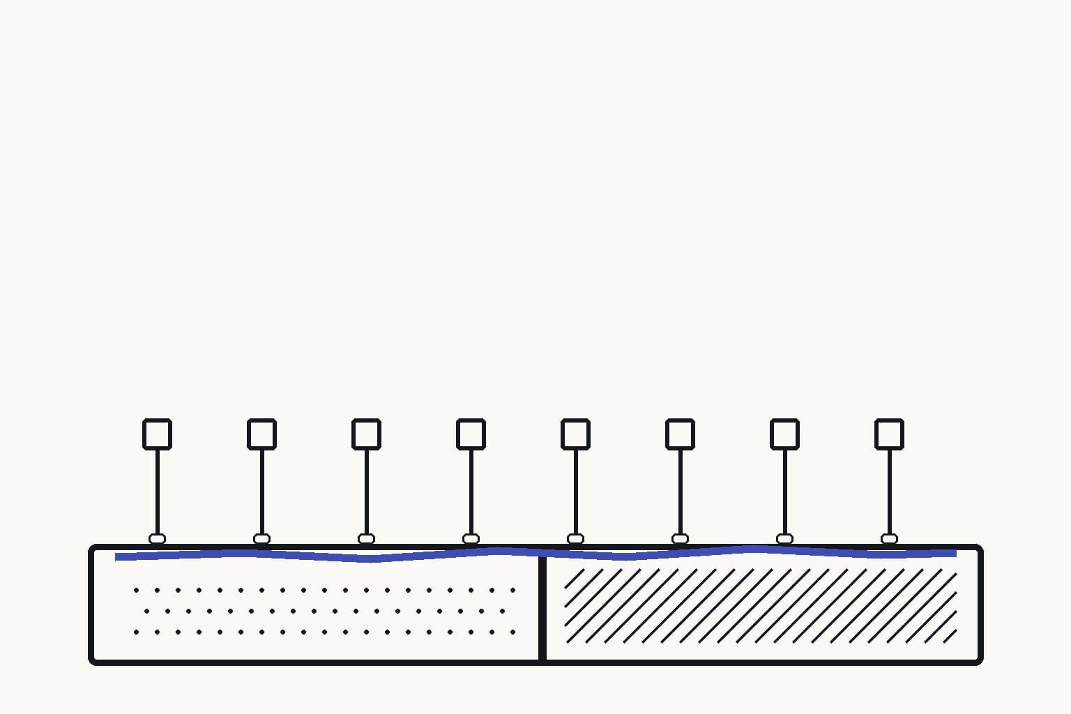
The method imposes the functional form. A cubic spline through three standard anchor observables — the (100) surface probing $c=8$, the (111) surface probing $c=9$, and the vacancy formation energy probing $c=11$ — is fixed by the boundary condition $P(12) = 0$. Linear continuation below $c=8$ predicts the error at $c=7$, which corresponds to the (110) surface energy. That observable is never fitted during field construction; it is predicted blind.

Each anchor samples a different coordination deficit relative to the bulk reference. Because the same coordination numbers recur across materials that share a crystal structure family, the spline transfers across properties within that family — surface energies, vacancy formation energies, and migration barriers — without additional DFT oracle calls. The correction is measured in the sense that geometry dictates the functional form and only the three knot values are empirical.

The r = 0.906 Result

The empirical test is strict blind prediction. Across 36 independent (model, material) combinations, the field predicts the signed error of the never-fitted (110) surface energy with Pearson correlation $r = 0.906$ ($p = 10^{-4}$, 95% confidence interval [0.82, 0.96]), using zero adjustable parameters.

The per-model breakdown is informative. CHGNet v0.4.2 achieves $r = 0.86$ ($p < 0.01$). MACE-MP-0 small achieves $r = 0.90$ ($p < 0.01$). MACE-MPA-0, trained on the larger OMat24 non-equilibrium dataset, achieves $r = 0.96$ ($p < 0.001$). MACE-MP-0 medium is the one non-significant case at $r = 0.47$ ($p = 0.10$). That exception matters: it bounds the field’s domain rather than refuting it. The OMat24-trained model performs best because its training distribution already samples more under-coordinated configurations, supporting the hypothesis that the field captures a real training-data bias rather than an accidental correlation.

An honest null is essential. Because (100), (111), and (110) facets of the same material are structurally correlated, a naïve permutation null would be too permissive. The reported null distribution, with mean $r = 0.44$, is generated by permuting within models across 10,000 draws, preserving the structural correlation. The measured $r = 0.906$ survives this conservative test.

At integer-scaled precision of $10^{-4}$ J/m$^2$, 26 of 36 cells improve strictly over the predict-zero baseline, with median residual dropping from 0.104 to 0.066 J/m$^2$. The number is 26, not 27 — a distinction that becomes important when the same pipeline is subjected to machine-checked proof.

Runtime Correction

The field inverts naturally into an additive correction energy:

$$E_{\text{corr}} = -\sum_i P(c_i).$$

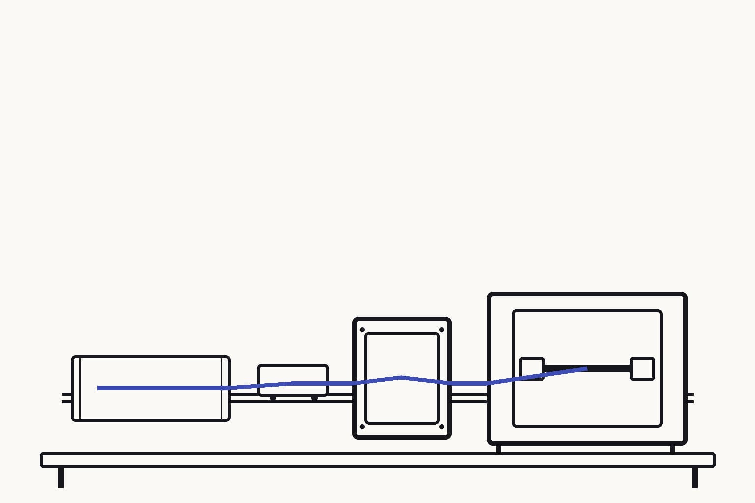
Because the field is negative where the model underpredicts — the typical case for defects and surfaces — the correction raises under-coordinated configurations toward the reference energy. Forces follow analytically from the chain rule, $F_{\text{corr}} = -\nabla E_{\text{corr}} = \sum_i P'(c_i) \nabla c_i$, so molecular dynamics conserves energy and structure relaxations follow proper gradients. Force accuracy was verified against numerical differentiation to $10^{-6}$ eV/Å on rattled slabs.

The correction layer deploys beside any existing uMLIP calculator without retraining its weights. Coordination computation is a local neighbor-list operation, so the overhead is small: 15.6% on CHGNet steps in the current Python implementation. A compiled pair-style overlay in LAMMPS would reduce that below 1%, because coordination reduces to a few floating-point operations per neighbor pair. Even with the present overhead, a corrected uMLIP remains many orders of magnitude faster than DFT.

Validation confirms selective correction. The fitted observables recover exactly in closure tests, demonstrating that the bond-counting field survives real structural relaxation. The blind (110) facet improves 6.5× for Ni (9.7% error to 1.5%) and 2.0× for Cu (28.0% to 13.7%). Bulk lattice constants are unchanged, because the correction vanishes identically at $c = 12$.

Machine-Checked Proof

Statistical validation has a well-known limitation: it cannot catch bugs in the analysis code, and it applies only to the samples tested. A formal verification layer is added. Every quantitative claim — ordering relations, correction bounds, and impossibility results — is encoded as a Lean 4 theorem over integer-scaled data carrying SHA-256 provenance of the source files. The formalization currently comprises 899 build-locked theorems and zero sorry proofs — Lean’s escape hatch for unproven claims. The count is generated directly from the open Lean source at build time.

The theorems fall into three categories. Ordering claims are inequality chains verified by the Lean kernel at fixed precision, not statistical summaries. Isotonic correction theorems implement the log-affine correction as a Lean function whose outputs the kernel checks against expected ordering properties. Impossibility theorems prove, with concrete counterexample witnesses, where no monotone correction can reconcile a model’s ordering with the reference ordering.

The kernel-rejected claim episode illustrates why this matters. A statistical filter initially accepted that 27 of 36 cells improved strictly. When submitted to Lean, the decide tactic refused to prove $813 < 813$; at $10^{-4}$ J/m$^2$ integer precision, one cell’s improvement margin was exactly zero. The corrected count is 26 of 36. A p-value does not know about integer rounding; the proof kernel does. In a pipeline where each false positive can cost weeks of synthesis effort, the distinction between statistical confidence and mechanical certainty is economically decisive.

Where Correction Fails, the Framework Proves Impossibility

A verification layer is only as useful as its boundary conditions. No claim is made that the field works everywhere; the framework proves where it cannot work. Three boundary conditions are formally established.

First, ranking inversions. When a model’s ordering disagrees with the reference ordering, a monotonicity impossibility lemma proves that no monotone correction can map both to their references simultaneously. The experimentalist receives not a vague uncertainty estimate but a machine-checked statement that the candidate cannot be rescued within the method.

Second, already-converged cells. Where the raw uMLIP error sits at the noise floor of the anchor observables — for instance, MACE-MPA-0 on certain surfaces — correction adds no value and is refused. The proof flags the redundancy before computational effort is wasted.

Third, outside the field’s domain. Environments that require second-shell structure or explicit electronic-structure treatment — planar faults, charged defects, strongly correlated oxides — are outside the first-shell coordination approximation. The framework proves the domain violation and reports the witness.

These impossibility proofs are not admissions of weakness. They are the feature that prevents the A-Lab pattern: systematic false positives propagating through an autonomous pipeline because no layer knew how to say no.

The Six-Step Loop

The field measurement, runtime correction, and formal verification layers close into a six-step discovery cycle:

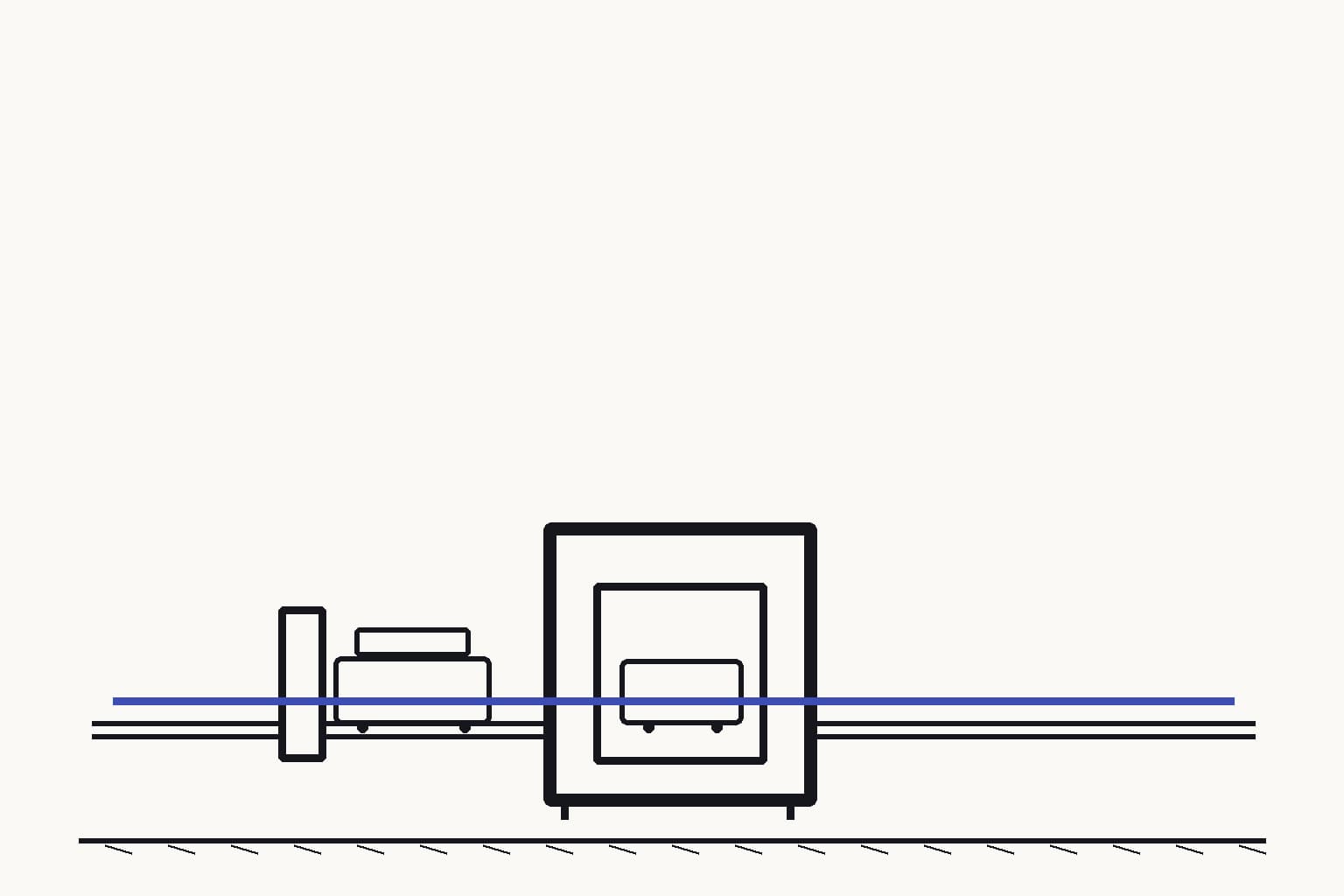
1. Simulate — run a uMLIP through the standard property pipeline: equation of state, surface slabs, vacancy supercells.
2. Identify — compare predictions to the 228-value provenance-annotated reference database.
3. Validate — check whether errors follow the environment error field; use the three anchors to predict a fourth blind observable.
4. Generate — construct the cubic spline $P(c)$ and deploy it as an additive correction with analytic forces.
5. Verify — submit every quantitative claim to the Lean 4 kernel; ordering claims become inequalities, correction bounds become isotonic theorems, failures become impossibility lemmas.
6. Improve — run the corrected calculator through the full pipeline. If correction succeeds, report corrected values with theorem certificates. If it fails, the impossibility proof tells the experimentalist why.

These certificates are no longer only a publication artifact. The field-domain gate, ranking-inversion gate, and barrier-underestimation conservatism check are now wired into the runtime policy engine and the promotion gate. When a prediction carries first-shell coordination data, the system checks whether every atom lies inside the measured field’s domain; out-of-domain atoms trigger a skip_correction action backed by FieldDomain.refusal_has_witness. When a candidate model is promoted, adjacent pairs in its reference and predicted rankings are checked for monotone rescuability; an inverted pair is downgraded automatically because inversion_defeats_monotone proves no monotone recalibration can rescue it. Barrier claims are checked against softened_barrier_underestimates and softening_never_hides_conductor. The mathematics that was proved in Lean now governs what reaches the lab.

Against DFT, the loop offers comparable defect-energy accuracy at many orders of magnitude higher speed. Against raw uMLIPs, it replaces uncontrolled systematic bias with a bounded, measured correction. Against delta-ML and fine-tuning, it eliminates per-system retraining because the spline transfers within a crystal-structure family. The practical consequence: a $10^6$-structure screening campaign needs no DFT calls, yet every candidate carries a provable accuracy boundary.

From Geometry to Climate Targets

The field is not an abstract mathematical device. It maps directly onto the defects, surfaces, and transition states that determine climate-critical material performance.

In cobalt-free lithium-manganese-rich cathodes, voltage fade is transition-metal migration from octahedral to tetrahedral sites — a hop whose barrier is underestimated when the transition state is under-coordinated. In earth-abundant halide solid electrolytes, ionic conductivity depends exponentially on the Li$^+$ migration barrier; a 60% barrier error changes predicted conductivity by roughly three orders of magnitude. In MOFs for direct air capture, humidity stability is governed by metal-linker hydrolysis at under-coordinated nodes. In electrochemical ammonia catalysts, N$\equiv$N cleavage occurs at surface defect sites. In lead-free perovskite absorbers, Sn$^{2+}$ oxidation and vacancy formation set the stability ceiling.

Every one of these properties is a coordination-dependent defect property. Every one is therefore within the domain where a measured error field can correct the prediction, or where an impossibility proof can flag the candidate as unsupported. The next part turns from the method to the targets: five material classes where correction plus verification could unlock 5–12 GtCO$_2$/year.

Footnotes